An oddity in the forward-forward algorithm
Introduction
Hinton shook the machine learning world with a novel way to train neural networks without backpropagation - the Forward-Forward algorithm. The backpropagation algorithm was a game changer when it was discovered in 1986 (which Hinton contributed to) and it has been pretty much been the only method used to train neural networks. As we started to realise how effective larger networks can be, we’ve poured in lots of computational resources and research into training larger and larger models. Today we have model that have up to half a trillion parameters. Most people have accepted that bigger is better.
While Hinton knows and agrees that larger nets are better, he challenges the idea that backpropagation is the only way to train these networks. The FF algorithm was designed from the ground up to forget about GPUs and digital computers. It was designed to work on analog computers - just charges doing math.
How does the Forward-Forward Algorithm work?
Instead of the conventional forward and backward passes of backpropagation, it uses two forward passes, one with positive (real) data and the other with negative data to learn using a contrastive approach. Each layer has its own objective function, with the goal of having high goodness for positive data and low goodness for negative data and the weight updates are done at each layer. This allows for layer-wise training.
The source and type of the negative data is one of the most important factors of this algorithm and the paper discusses a few ways that this can be done. This also influences how we perform inference and evaluate the model. There are also several open questions such has what other loss functions or activation functions can be used, and how it can be extended for other use cases.
Before diving into questions about the FF algorithm, lets go over some related works of how we can train neural networks without backpropagation.
Signal Propagation (sigprop)
Signal propagation acts as a precursor to the forward-forward algorithm where it is considered to be the least constrained method for learning and said to provide better performance, efficiency and compatibility compared to previous alternatives to backpropagation such as Feedback Alignment and Local Learning (Kohan et al., 2022). The idea of sigprop is to reuse the forward path to map an initial learning signal into targets at each layer for updating parameters, and bring the input data and targets close together after each layer of training. The network is fed with two inputs: the data and the learning signal. The learning signal is defined as explicit labels, as used in supervised learning.
2.1.1 Training
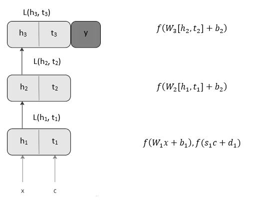
Figure 1 provides an overview of the neural network with 2 hidden layers and how the data and learning signals are used as inputs to the network.

Figure 1: model of signal propagation with 2 hidden layers
\(x\) and \(c\) are the input and learning signals respectively which are fed into the first layer of the network. These 2 inputs are different in shape; \(c\) is obtained using a one hot encoding method of the label. \(W_i\) and \(b_i\) are the weight and bias for layer \(i\). \(S_1\) and \(d_1\) are the weight and bias for the target generator. The function \(f\) is a non-linear activation function which will transform the inputs and produce an output labelled \(h_1\) and \(t_1\) respectively with the same shape. The outputs are given in the equation below.
\[h_1 ,t_1 =f(W_1x + b_1) , f(S_1c_m+ d_1)\]\(t_1\) is the output target for the first hidden layer \(h1\) where the loss \(L1(h1, t1)\) is calculated between them for the training of the first layer. There are many choices for a loss function, Hebbian for gradient algorithms and SGD, ADAM for optimizing algorithms. Next, \(h_1\), \(t_1\) are fed into the next hidden layer where they will be used for training in that layer. The forward pass continues this way until the final layer is reached, producing outputs with the equations below.
\[[h_2 , t_2] =f(W_2[h_1,t_1] + b_2)\] \[[h_3 , t_3] =f(W_3[h_2,t_2] + b_2)\]Each layer locally compares its output and the output target using a loss function to update its parameters. Upon reaching the final layer, it performs one last update to its parameters and finally produces a prediction \(y\).
\[y = O(h_3, t_3)\]Where \(O\) is a comparison function such as dot product or L2 distance. Overall, sigprop allows the network to learn to process the input and produce an output. Simultaneously, it learns to make an initial learning signal into a useful training target at each layer.
2.2 Forward-Foward
The Forward-Forward algorithm operates similarly to sigprop by replacing the forward and backward passes of backpropagation with two forward passes. However, the difference here is that sigprop aims to bring the input and the target labels close together while maximizing the distance of other dissimilar inputs and its corresponding target. The forward-forward algorithm instead have a “positive pass” and a “negative pass” with opposite objectives that are fed into the network. The positive pass operates on real data and adjusts the weights of the network to increase the goodness of each layer, while the negative pass operates on negative data and adjusts the weights to reduce goodness. The positive data consists of an image with the correct label, while the negative data consists of an image with the incorrect label, which is randomly assigned. The goodness of a layer can be quantified using a sum of squares of the activities in the ReLU of that layer. The objective of the forward pass is for the goodness to be well above a predefined threshold value, and the inverse for negative pass. The model should then be able to classify positive and negative inputs in the following equation:
\[p(positive) = \sigma(\sum_j y_j^2-\theta)\]Where the probability of an input being positive is the logistic function of the goodness minus a predefined threshold.
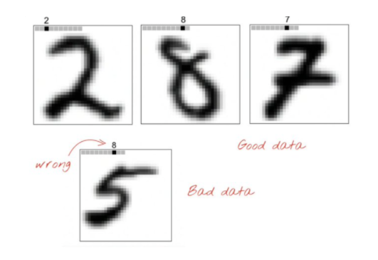
An example of labelling of the positive and negative data is given below. The labels are embedded into the original image using a one-hot encoding in the top left corner of the image (refer to Figure 2).

Figure 2: Positive and Negative Labelling of the data
As seen in figure 2, positive data are labelled appropriately using one-hot encoding to the first 10 pixels of the image, while the negative data are encoded into the image by randomly assigning a label from 0 to 9 to the images.
The oddity
While implementing my understanding of the algorithm, I noticed that there was one area that all other implementations posted online seem to overlook - the selection/preparation of “negative data”. With regards to the MNIST example in the paper, Hinton mentions that the negative data can be mislabeled data (like seen in figure 2).
However, this is what we see in the training loop of the official Keras implementation:
random_y = tf.random.shuffle(y)
x_neg, y = tf.map_fn(fn=self.overlay_y_on_x, elems=(x, random_y))
What is happening here is that they are trying to create the negative data by ******randomly****** shuffling y (true labels) then overlaying the new random number onto the input image as the first 10 pixels (as seen in figure 2).
What they (and many others) have overlooked is that a random shuffle DOES NOT guarantee that the old value and the new value at a particular index of are different!
In fact roughly 10% of the data will be the same as before! Try running this code to see for yourself:
import numpy as np

#number of overlaps each run
overlaps = []

for _ in range(100):
    # array of 60000 random numbers from 0 to 9
    y = np.random.randint(0, 10, 60000)

    # copy the array
    y_copy = y.copy()

    #check the distribution of the numbers
    np.bincount(y)

    # shuffle the array
    np.random.shuffle(y_copy)

    #count the number of times the same number appears in the shuffled array
    overlaps.append(sum(y == y_copy))
    # print(f"Overlaps: {sum(y == y_copy)}")

# print the average number of overlaps
print(f"Average number of overlaps: {np.mean(overlaps)}")
#print the standard deviation of the overlaps to 2 decimal places
print(f"Standard deviation of overlaps: {round(np.std(overlaps), 2)}")
#print the percentage of overlaps rounded to 2 decimal places
print(f"Percentage of overlaps: {round(np.mean(overlaps)/60000*100, 2)}%")
>>> Average number of overlaps: 5988.51
>>> Standard deviation of overlaps: 74.55
>>> Percentage of overlaps: 9.98%
What this means is that by choose to use a random shuffle, 10% of the negative data that is fed to the network is actually the same as the positive data!! So the negative data would cancel out the positive data and no learning happens for that example.
BTW: Could someone explain why this shuffling causes a 10% overlap?
Hypothesis: A perfect randomisation should roughly yield a 10% boost in accuracy
I attempted several methods to compare the model accuracy from merely shuffling the data against carefully removing or reducing the overlaps. Surprisingly, just a simple shuffle worked the best.
Experiments
- Remove the duplicates in the positive and negative data. This constituted to about 10% loss in training data.

- Assignment of the negative label from the randomisation of labels other than the correct label. If the true label is 5, then we randomly pick anything other than 5. This was my initial understanding of the paper.

- Select the duplicates in the positive and negative data, and randomise the negative label again.

- Perfect random derangement - keep only 5000 training examples for each label then perform a random derangement.
The neural network used to perform training for all experiments consisted of two hidden layers with 500 neurons each, and was trained for 1000 epochs batch-wise and a learning rate of 0.03 for the Adam optimizer. The threshold parameter for goodness was set to 2. All the experiment results were also averaged over 20-30 runs each.
Results
| x | Random shuffle | Experiment 1 | Experiment 2 | Experiment 3 | Experiment 4 - random shuffle | Experiment 4 - random derangement | |||||||
|---|---|---|---|---|---|---|---|---|---|---|---|---|---|
| Train Error | 0.0708 | 0.0748 | 0.0737 | 0.0741 | 0.07125302 | 0.07499802 | |||||||
| Test Error | 0.0711 | 0.0731 | 0.0730 | 0.0726 | 0.07032502 | 0.07235502 |
I expected experiment 4 to perform the the best. In experiment 4, the perfect derangement method was compared against the random shuffle and the results were roughly the same! This was really confusing. The model that was fed with better data performed very slightly worse than another model that had arguably 10% less data?!
Further investigations
At this point, more digging needs to be done to understand the FF algorithm. I feel that the random shuffle might be better than expected because it might have some regularisation effects similar to dropout.
I also wonder if there is some threshold for the number of hidden layers and parameters after which learning stops. Perhaps the net I used for the experiments were too large to notice the effects of the differences in data.
Despite the issue with the negative data, there are many other interesting questions to explore. I also tried to look into other suitable loss functions and felt that an (inverse) cosine similarity loss function might work. In the paper, Hinton asks us to think about the activations as a vector that has some orientation. So by contrasting the orientation from the positive data and the negative data we could update the weights. However, from some basic experiments, this did not yield good results. The model stops learning after the first layer.
There is also a question of how the FF algorithm can be adapted to convolutional neural networks. The FF algorithm does layer-wise weight updates so I wonder how the convolutional layers can be trained using this method…
If you have any thoughts on this matter please reach out to me!
Enjoy Reading This Article?
Here are some more articles you might like to read next: