Disproving Norine's conjecture
I started working on this research project in May 2021 under SUTD’s UROP programme with one other undergraduate student, Anirudh Srinivason, under the guidance of a professor. This is a summary of our work and the results we found.
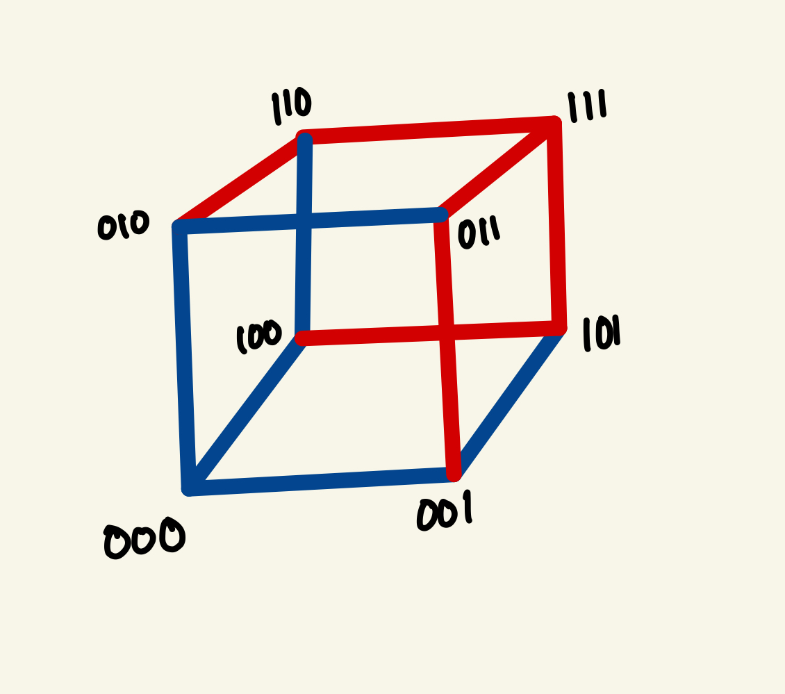
🧠 Conjecture: For any cube in 3 or more dimensions, there exists an antipodal 2-colouring
of edges such that there exists a monochromatic path from one vertex to the opposite vertex.
Some definitions:
- N-cube / hypercube graph - a graph of a cube in N dimensions. 2-cube is the square, 3-cube is the cube, 4-cube is known as a tesseract. It is hard to visualise cubes in 5 or more dimensions so we just trust the math.
- edge/vertex 2-colouring - it means to colour edges or vertices of a graph using only 2 colours such that no two adjacent edges or vertices are of the same colour. This is also known as a bi-partition of a graph. Usually, the colours red and blue are used to colour the edges but any colour or any kind of label would work.
- antipodal edge colouring - this means to use opposite colours for opposite edges.

</figure>
- path - while there may be many interpretations and definitions for what a path in a graph may be in the discrete mathematics and computer science world, in our case, a path is a sequence of edges from one vertex to another. Specifically, the path we are looking for is one that can take us from a starting vertex to its opposite vertex.
- Monochromatic path - A path that only consists of edges of a single colour (all red/blue)
- Number of edges in an N-cube - \(2^{N-1}N\)
- Number of vertices in an N-cube - \(2^N\)
- Diameter of an N-cube - \(N\)
Since we are dealing with a conjecture we could either prove or disprove it. Currently, this conjecture has been verified to be true for up to N = 7 (7-cube) by hand, but not a lot of promising results have been published to show that the conjecture is true. One way to disprove is to find a counter example.
Initially when I started exploring this topic and tried out some small examples, my gut feeling was that the conjecture is probably true. However, our professor felt otherwise and suggested exploring ways to disprove. It does not matter if there are an infinite number of examples to show that the conjecture is true, we just need to find one counter example to disprove the conjecture. So we tried our best to find ways to disprove the conjecture.
Thus, the aim of this project was to find a particular colouring of a hypercube graph such that no monochromatic paths exists between any pair of antipodal nodes.
Ant Colony Optimisation
It can be tempting to imagine how hypercube graphs look like in our head but it can often be confusing and misleading. Thus, as a warm-up problem, we worked on writing code to generate and traverse hypercubes. We first tried to try to generate random hypercubes that follow the antipodal colouring rule and pick random starting points to see if it was possible to get from a start vertex to an opposite vertex with a modified version of the ant colony optimisation algorithm.
TLDR - Ant Colony Optimisation: It is a heuristic that is used to solve the travelling salesman problem. The idea is to place a bunch of ants at a starting vertex of a graph and let ants traverse the graph while leaving a pheromone trail on the edges based on the “goodness” of that edge to get towards the end vertex, so that other ants may take advantage of the exploration done by an ant. This helps to converge to the solution with less computational effort than an exhaustive search, however this may not work all the time. It is just an approximate solution.
By averaging the results of thousands of runs of this algorithm on random graphs, we can get an understanding of how “hard” it is for the ants to find a monochromatic path. This can thus serve as a baseline in our search to find a counter-example. The hardness of the path can be characterised by the length of the path taken, the number of iterations needed, and several other factors.
We tried several simple coloring schemes to understand which colourings are more “adversarial”.
- Random colouring: Simply traverse the graph and coloring the edges randomly while adhereing to the antipodal colouring rule
- Layer-by-layer colouring: Starting from the zero-vector, we can define the first layer to be all the edges connected to the zero-vector. Then the second layer would be all the (uncoloured) edges connected to all the neighbours of the zero-vector. The subsequent layers follow a similar pattern. Again, the antipodal edge coloring rule must be obeyed so some sensible adjustments to the layer-wise colouring will have to be made. The idea here is to use alternating colours for each layer to try to force colour changes.
- Dynamic-Layer-wise colouring: Similar to the layer-wise colouring, but instead we use larger chunks of layers to be the same colour
Thinking adversarially
We want to define a coloring such that no matter where we start, we would like to force at least one colour change at the start vertex and at the end vertex. One thing to note about any colouring scheme for hypercubes is that it is highly symmetrical - colouring half of all the edges will end up setting the colour for the other half of the cube due to the antipodal colouring rule. Since we need to think about a colouring scheme that is agnostic to the starting point, it helps to start thinking from the point of view of sub-regions of a hypercube.
Getting serious: Coding theory
Coding theory mainly deals with the study of Error-Correcting Codes (eg. ECC memory). It makes use of mathematical structures such as vector spaces and matrices to represent codes and encode/decode messages. For example, a binary code can be represented as a vector space over the finite field of two elements (0 and 1), where the vectors are binary words of a fixed length.
One interesting mathematical object used in coding theory is the hypercube. The n-dimensional hypercube is a graph with 2^n vertices, each of which represents a binary word of length n. Two vertices are adjacent if they differ in exactly one position (Hamming distance = 1). The hypercube has the property that any two vertices are connected by a path of length equal to their Hamming distance. This property is used to analyze the performance of certain codes, such as the Hamming code.

(Visualisation of a 4-cube. Source: Wikipedia)
Interlude: Why are perfect codes so darn perfect?
💁🏼♀️: Alright, listen up, sweetie, perfect codes are like the Beyoncé of coding theory: flawless, fierce, and highly sought-after. And when it comes to perfect codes, the Golay code is the queen bee.
The Golay code is a binary linear code that can correct up to three errors in a block of length 23, while using only 12 redundancy bits. That's like having a superhero that can save the day with minimal effort, while looking cool doing it.
But here's the kicker: the Golay code is not just any perfect code, it's a Type II binary code, which means it has some special mathematical properties that make it even more awesome. For example, it has a unique triply even weight distribution, which is like having the perfect body shape in the coding world.
So, yeah, perfect codes are pretty amazing, and the Golay code is the queen of them all.
Credit: Sassy ChatGPT
Extended Binary Golay Code (Not a perfect code!)
The binary Golay code has many desirable properties such as Hamming Balls, symmetry and the idea of codewords. However, extending the \(G_{23}\) by 1 parity to bit to make it \(G_{24}\) gives us other desirable properties.
- There are exactly \(2^{12}\) (4096) codewords (and Hamming balls).
-
Every edge in the hypercube is contained within exactly 1 hamming ball
- However, this does not mean every vertex is contained within exactly 1 hamming ball
- If we can define a coloring within each Hamming ball such that regardless of the starting vertex within a hamming ball, we can ensure that there will have to be at least one colour change to “leave” the hamming ball, then we can simplify the problem to the subspace of codewords.
Here is an example of how we can colour a single Hamming Ball:

In there are 4 layers of edges from the centre of each hamming ball (the codeword). We can colour the edges in each layer with alternating colours. This ensures that there will be at least one colour change at the start vertex and at the end vertex. It is also important to note that exactly half of the codewords will have 1 in the last bit, and the other half will have 0 in the last bit. This allows us to categorise the hamming balls into two groups (red and blue). For example, the above example can be considered as a red hamming ball. A blue hamming ball would have the opposite colouring scheme.
How many vertices are contained within a hamming ball? Lets break it down by layers:
- 1st layer: 1 vertex (codeword)
- 2nd layer: \(\choose{24}{1} = 24\) vertices
- 3rd layer: \(\choose{24}{2} = 276\) vertices
- 4th layer: \(\choose{24}{3} = 2024\) vertices
- 5th layer: \(\choose{24}{4} = 10626\) vertices
Now we can consider paths from one hamming ball to the opposite hamming ball. The diameter of the cube is 24 and the diameter of a hamming ball is 4. Therefore, the shortest path to the opposite vertex would mean 5 other hamming balls would have to be visited. According to the literature on Golay codes, there will be 253 oppositely coloured hamming balls that are in contact with each hamming ball. Conversely, there will be 6 hamming balls that “share” each vertex in the last layer of the hamming ball. What all of this means for us is that, from a hamming ball perspective, the path between two antipodal vertices will have to pass through 5 other hamming balls that are alternating between red and blue. This must be it right? Well, not quite….
Learning the truth
In order to test out this theory, we needed some serious compute. Thankfully, we were able to get access to the National Supercomputing Centre in Singapore (NSCC) to run our experiments. It was a bit of a learning curve to get used to the NSCC’s HPC system, like writing and submitting jobs to the queue, but we managed to get it done. It takes a whopping ~500gb of RAM to store the entire hypercube, so we had to be careful with our memory usage.
After successfully generating the colouring for the 24-cube, we ran some tests to see if our theory was correct. Unfortunately, we discovered that the hamming balls behaved differently from what we expected. Ultimately, the problem was with understanding what happens at the last layer of each hamming ball. The 24-cube is known as the extended binary Golay code because it is able to detect up to 4 error but only correct up to 3 errors. The same analogy can be applied to our situation. The truth is that we later found out was that the 0-codeword hamming ball is actually in contact with 759 hamming balls. The 759 can be futher broken down to 253 red hamming balls and 506 blue hamming balls. This means that hamming balls of the same colour are not completely isolated from each other.

Moving forward
After learning from that failure, we tried a few more ideas. We tried to fall back to the \(G_{23}\) and tried some ideas but they also had some flaws. After spending roughly 1 year on this project, trying our best to disprove the conjecture, I am left with the feeling that perhaps the conjecture is true but just very difficult to prove. We tried the most adversarial approaches we could think of, but we were unable to disprove the conjecture. This is a very interesting problem and I hope that someone will be able to prove it one day!
Enjoy Reading This Article?
Here are some more articles you might like to read next: