SHAP - by Portcast.io
import numpy as np
import pandas as pd
import pickle
Reading the data
data = pd.read_csv('sample_data.csv')
Importing the model
filename = 'eta_model.sav'
eta_model = pickle.load(open(filename, 'rb'))
features = [
      'speed_nm',
      'predicted_distance_left',
      'simple_predicted_distance_over_speed',
      'ports_distance',
      'schedule_eta',
      'congestion_index'
      ]
Computing shap values
import shap
explainer = shap.TreeExplainer(eta_model)
X = data[features]
shap_values = explainer.shap_values(data, approximate=True)
Global Interpretability
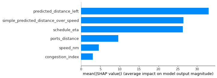
The idea behind SHAP feature importance is simple: Features with large absolute Shapley values are important. Since we want the global importance, we sum the absolute Shapley values per feature across the data. We sort the features by decreasing importance and plot them. The following figure shows the SHAP feature importance for the random forest trained before for predicting the ETA.
shap.summary_plot(shap_values, X, plot_type="bar")

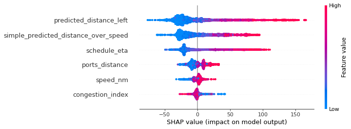
The summary plot combines feature importance with feature effects. Each point on the summary plot is a Shapley value for a feature and an instance. The position on the y-axis is determined by the feature and on the x-axis by the Shapley value. The color represents the value of the feature from low to high. Overlapping points are jittered in y-axis direction, so we get a sense of the distribution of the Shapley values per feature. The features are ordered according to their importance.
shap.summary_plot(shap_values, X)

explained_obj = explainer(X)
You can cluster your data with the help of Shapley values. The goal of clustering is to find groups of similar instances. Normally, clustering is based on features. Features are often on different scales. For example, height might be measured in meters, color intensity from 0 to 100 and some sensor output between -1 and 1. The difficulty is to compute distances between instances with such different, non-comparable features.
SHAP clustering works by clustering on Shapley values of each instance. This means that you cluster instances by explanation similarity. All SHAP values have the same unit – the unit of the prediction space. You can use any clustering method. The following example uses hierarchical agglomerative clustering to order the instances.
The plot consists of many force plots, each of which explains the prediction of an instance. We rotate the force plots vertically and place them side by side according to their clustering similarity.
shap.initjs()
shap.force_plot(explainer.expected_value, explained_obj.values[:1000,:],data.iloc[:1000,:], plot_cmap="DrDb")
Enjoy Reading This Article?
Here are some more articles you might like to read next: